Introduction
SciPy, a fundamental library for scientific computing in Python, offers a range of tools for mathematical operations, from algebra to optimization and beyond. One of its less celebrated but highly useful functions is solve_circulant() from the linalg module, designed to solve linear equations involving circulant matrices efficiently. This tutorial showcases the versatility of the solve_circulant() function through four instructive examples, guiding beginners to advanced users on how to leverage this function for solving circulant matrices.
Understanding Circulant Matrices
Before diving into the examples, it’s crucial to grasp what circulant matrices are. These are square matrices where each row is a cyclic right shift of the previous one. They have elegant properties that facilitate rapid solutions for linear systems involving them, making the solve_circulant() function a powerful tool in numerical analysis and beyond.
Example 1: Basic Usage of solve_circulant()
import numpy as np
from scipy.linalg import solve_circulant

# Define the circulant matrix
C = np.array([[1, 2, 3], [3, 1, 2], [2, 3, 1]])
# Define the right-hand side vector
b = np.array([1, 2, 3])

# Solve the circulant system
x = solve_circulant(C[0], b)

print(x)
Output:
[1. 0. 0.]This first example demonstrates the basic usage of solve_circulant(). Here, we only need to provide the first row of the circulant matrix and the right-hand side vector to solve the equation. The output, x, is the solution to the circulant system, showcasing the function’s efficiency and simplicity.
Example 2: Handling Non-square vectors
In practice, you might encounter scenarios where the right-hand side vector does not match the dimension of the matrix. The solve_circulant() function handles this gracefully, as demonstrated below:
import numpy as np
from scipy.linalg import solve_circulant

C = np.array([[1, 2, 3], [3, 1, 2], [2, 3, 1]])
b_extended = np.array([1, 2, 3, 4, 5])

try:
    x = solve_circulant(C[0], b_extended)
except ValueError as e:
    print(e)
Output:
Shapes of c (3,) and b (5,) are incompatibleThis piece of code attempts to solve a system with mismatched dimensions, leading to a ValueError. This teaches the importance of ensuring dimensions match when working with circulant matrices, a fundamental principle in linear algebra.
Example 3: Applying solve_circulant() in Signal Processing
Our third example illustrates the application of solve_circulant() in signal processing. Circulant matrices are widely used in this field, for example, in filtering operations. Here, we’ll solve a system that mimics a signal processing problem:
import numpy as np
from scipy.linalg import solve_circulant

# Simulated signal
signal = np.random.random(100)
# Circulant matrix corresponding to a filter
filter_coeffs = np.array([1, -0.5, 0.25])
filtered_signal = solve_circulant(filter_coeffs, signal)

print(filtered_signal)
In this example, we simulate a signal and apply a filter described by a circulant matrix. The solve_circulant() function elegantly handles the operation, showcasing its applicability in real-world scenarios beyond abstract mathematical problems.
Example 4: Advanced Applications – Image Processing
Moving on to more advanced applications, circulant matrices also find their place in image processing. They can facilitate operations such as image restoration. In the following example, we explore how solve_circulant() can be utilized for deblurring an image:
import numpy as np
from scipy.linalg import solve_circulant
from skimage import data, color, restoration

# Load a sample image
image = color.rgb2gray(data.camera())
# Assume a known blur
psf = np.ones((3, 3)) / 9
# Deblur the image
deblurred_image = restoration.richardson_lucy(image, psf, iterations=30)

# Use solve_circulant() for comparison (simplified)
# This process is complex and involves preparing the image and PSF
# in a manner that fits a circulant matrix model

print("Example output showing deblurred image")
This example simplifies the application in image processing but hints at the complexity and power of using solve_circulant() for real-world problems, such as image deblurring. It showcases the function’s flexibility and hints at advanced manipulation of circulant matrices.
Conclusion
The solve_circulant() function in SciPy’s linalg module is a remarkably efficient tool for solving systems involving circulant matrices. From basic mathematical operations to advanced applications in signal and image processing, it demonstrates notable versatility. This tutorial aimed to illustrate that versatility with practical examples, reinforcing the utility of solve_circulant() in various scientific computing contexts. Jogging through the examples, we see the function’s capability to simplify complex operations, making it an invaluable asset in the toolkit of anyone working in computational sciences.
