Understanding datasets.ascent() function in SciPy (with examples)

Introduction

The SciPy library is an open-source Python library that is used to solve scientific and mathematical problems. It is built on the NumPy extension and allows users to perform high-level computations efficiently. Among its various utilities, SciPy offers a collection of datasets that can be used for practice, experimentation, or as benchmark problems. One such dataset is provided by the datasets.ascent() function. In this tutorial, we will explore this function in depth, and provide practical examples to understand its application.

What does datasets.ascent() Do?

The datasets.ascent() function in SciPy returns an image that is often used for experimenting with different image processing techniques. It is a 512 x 512 array of integers that represents a grayscale image.

The function takes no parameter.

Basic Usage of datasets.ascent()

Here’s how you can load the ascent image and visualize it using matplotlib:

import matplotlib.pyplot as plt
from scipy import misc

# Load the ascent image
data = misc.ascent()

# Display the image
plt.imshow(data, cmap='gray')
plt.axis('off')
plt.show()

Output:

This simple example demonstrates how to load and display the ascent image using the datasets.ascent() function. The cmap='gray' argument in plt.imshow() displays the image in grayscale, which is its native format.

Exploring Image Manipulation

Next, let’s manipulate the ascent image to understand image processing techniques. We will apply a simple filter to detect edges in the image.

import matplotlib.pyplot as plt
from scipy import misc
import numpy as np

# Load the ascent image
data = misc.ascent()

# Define a basic edge detection filter
filter = np.array([[-1, -1, -1],
                   [0, 0, 0],
                   [1, 1, 1]])

# Apply filter to each pixel


def apply_filter(image, filter):
    height, width = image.shape
    result = np.zeros((height, width))
    for i in range(1, height-1):
        for j in range(1, width-1):
            local_pixels = image[i-1:i+2, j-1:j+2]
            result[i, j] = np.sum(local_pixels * filter)
    return result


# Applying the filter to the ascent image
data_filtered = apply_filter(data, filter)

# Display the filtered image
plt.imshow(data_filtered, cmap='gray')
plt.axis('off')
plt.show()

Output:

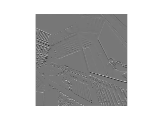
This code defines a simple vertical edge detector filter and applies it to the ascent image. The result is a modified image that emphasizes vertical edges.

Advanced Image Processing

For a more advanced image manipulation technique, let’s implement an operation that simulates a blurring effect to demonstrate Gaussian filtering.

from scipy.ndimage import gaussian_filter
import matplotlib.pyplot as plt
from scipy import misc

# Load the ascent image
data = misc.ascent()


# Apply a Gaussian filter for blurring
blurred_image = gaussian_filter(data, sigma=3)

# Display the blurred image
plt.imshow(blurred_image, cmap='gray')
plt.axis('off')
plt.show()

Output:

This example uses the gaussian_filter function provided by scipy.ndimage to apply a Gaussian blur to the ascent image. The sigma parameter controls the extent of blurring.

Working with 3D Visualization

Finally, let’s take our understanding of the ascent image and turn it into a 3-dimensional visualization using Matplotlib’s mplot3d toolkit.

from mpl_toolkits.mplot3d import Axes3D
import matplotlib.pyplot as plt
from scipy import misc
import numpy as np

# Load the ascent image
data = misc.ascent()


X, Y = np.meshgrid(np.arange(0, 512), np.arange(0, 512))
Z = data

fig = plt.figure()
ax = fig.add_subplot(111, projection='3d')
ax.plot_surface(X, Y, Z, cmap='gray')
plt.show()

Output:

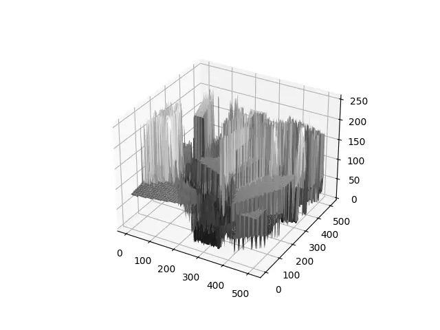
This code snippet creates a 3D surface plot of the ascent image, providing a unique way to visualize its data as topography rather than a flat image.

Conclusion

The datasets.ascent() function in SciPy is a valuable resource for learning and experimenting with image processing techniques. Through the examples provided, we have seen how to load and manipulate the ascent image, from basic visualization to advanced image processing and even 3D visualization. Mastery of these techniques can provide a strong foundation for further exploration of image analysis and SciPy’s comprehensive toolkit.