NumPy: How to draw samples from a Beta distribution (3 examples)

Introduction

NumPy is a cornerstone of the Python data science ecosystem, offering robust methods for numerical computation. Among its powerful features is the ability to sample from various statistical distributions, including the Beta distribution, which is particularly useful in Bayesian analysis and other fields of statistical modeling.

This article explores how to draw samples from a Beta distribution using NumPy with three practical examples. We will start from the basics and gradually delve into more complex scenarios, showcasing the versatility of NumPy for statistical simulations.

Understanding the Beta Distribution

Before jumping into the examples, let’s briefly understand what the Beta distribution is. The Beta distribution is a continuous probability distribution defined on the interval [0, 1] and parameterized by two positive shape parameters, \\(\alpha\\) and \\(\beta\\). It is widely used in Bayesian analysis due to its flexibility in modeling phenomena whose outcomes are probabilities or proportions.

Example 1: Basic Sampling

The simplest form of drawing samples from a Beta distribution involves specifying the \\(\alpha\\) and \\(\beta\\) parameters. The code snippet below demonstrates how to generate 100 samples from a Beta distribution with \\(\alpha=2\\) and \\(\beta=5\\) using NumPy’s \texttt{numpy.random.beta}\ function.

import numpy as np

# Set the seed for reproducibility
np.random.seed(42)

# Generate samples
samples = np.random.beta(a=2, b=5, size=100)

# Display first 5 samples
print(samples[:5])

This code yields an array of samples, like so:

[0.35367666 0.24855807 0.41595909 0.15996758 0.55028308]

Example 2: Visualizing the Distribution

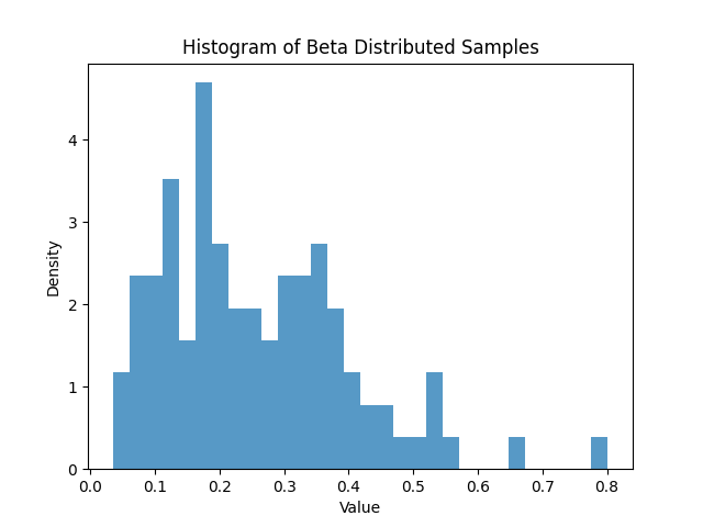
After generating the samples, it’s beneficial to visualize the distribution to understand its shape and spread. The following example employs Matplotlib to create a histogram of the Beta distribution samples generated previously. Firstly, ensure you have Matplotlib installed:

pip install matplotlib

Then, use this code snippet to create a histogram:

import matplotlib.pyplot as plt
import numpy as np

# Set the seed for reproducibility
np.random.seed(42)

# Generate samples
samples = np.random.beta(a=2, b=5, size=100)

# Plotting the samples
plt.hist(samples, bins=30, density=True, alpha=0.75)
plt.title('Histogram of Beta Distributed Samples')
plt.xlabel('Value')
plt.ylabel('Density')
plt.show()

This will produce a histogram as follows:

Example 3: Advanced Sampling with Different Parameters

Building upon the basics, let’s explore how to generate samples from Beta distributions with varying alpha and beta parameters to simulate different scenarios. The following code demonstrates generating samples from three different Beta distributions and visualizing them on the same plot for comparison.

import numpy as np
import matplotlib.pyplot as plt

# Generating samples from different Beta distributions
a_b_pairs = [(0.5, 0.5), (5, 1), (1, 3)]

for a, b in a_b_pairs:
    samples = np.random.beta(a, b, 1000)
    plt.hist(samples, bins=30, density=True, alpha=0.75, label=f'\alpha={a}, \beta={b}')

plt.title('Comparing Beta Distributions')
plt.xlabel('Value')
plt.ylabel('Density')
plt.legend()
plt.show()

Output:

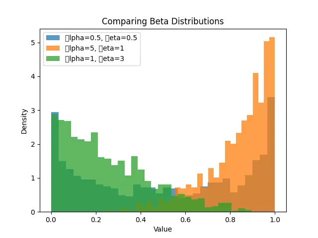
This comparative visualization helps in understanding the impact of varying \\(\alpha\\) and \\(\beta\\) parameters on the shape of the Beta distribution.

Conclusion

Through three progressively advanced examples, we have seen how NumPy can be utilized to draw samples from a Beta distribution and the importance of visualizing these samples. The ability to generate and analyze such distributions is essential for statistical modeling, particularly in fields like Bayesian inference. The flexibility of NumPy makes it an invaluable tool for both beginners and advanced users in the realm of data science.