SciPy: Using fft.hfft2() function (4 examples)

The SciPy library, a cornerstone of scientific computing in Python, offers a multitude of functions for fast Fourier Transformations (FFT), which are essential in fields like signal processing, image analysis, and more. Among these functions, fft.hfft2() is a powerful tool for computing the 2-dimensional FFT of a real array. This tutorial aims to elucidate the usage of fft.hfft2() through four progressive examples, guiding both beginners and advanced users in harnessing this function effectively.

Introduction to FFT and fft.hfft2()

Before diving into the examples, let’s understand what FFT is and what fft.hfft2() specifically does. FFT is an algorithm to compute the Discrete Fourier Transform (DFT) and its inverse, offering significantly improved computational speed compared to direct DFT calculations. The fft.hfft2() function in SciPy extends this capability to 2-dimensional data, particularly useful for processing images or 2D signals, while specifically focusing on real input data.

Example 1: Basic Usage of fft.hfft2()

This example demonstrates the basic usage of fft.hfft2() on a simple 2-dimensional array. The goal here is to understand how to apply the function and interpret its output.

import numpy as np
from scipy.fft import hfft2

# Creating a simple 2D real array
array = np.random.random((4, 4))

# Applying hfft2
result = hfft2(array)

# Displaying the output
print(result)

Output (vary):

[[ 9.25676528 -1.81060187 -0.30083537  1.98589321 -0.30083537 -1.81060187]
 [-1.31392544 -1.33195886 -0.42588379 -2.22549162  2.61120431  0.13747348]
 [-0.14935788 -0.72956733  1.887737    0.14164221  1.887737   -0.72956733]
 [-1.31392544  0.13747348  2.61120431 -2.22549162 -0.42588379 -1.33195886]]

The output will be a 2-dimensional complex array. As the input is real, the complex values provide insights into both the amplitude and phase of different frequency components present in the data.

Example 2: Analyzing Image Data

Shifting our focus to more practical applications, this example explores how fft.hfft2() can be used to analyze the frequency components of an image. This technique is pivotal in areas like image compression and noise filtering.

import matplotlib.pyplot as plt
from scipy.fft import hfft2, ihfft2
import numpy as np

# Loading an image
image = plt.imread('example_image.jpg')
# Converting to grayscale
gray_image = np.mean(image, axis=-1)

# Applying hfft2
frequencies = hfft2(gray_image)

# Visualizing the frequency domain representation
plt.imshow(np.log(np.abs(frequencies)), cmap='gray')
plt.title('Frequency domain representation')
plt.colorbar()
plt.show()

The visualization reveals how different frequencies contribute to the overall image, with higher frequencies often corresponding to edges and fine details.

Example 3: Filtering in Frequency Domain

Moving towards more complex applications, this example shows how one can perform frequency domain filtering to enhance or suppress specific features in image data.

from scipy.fft import hfft2, ihfft2
import numpy as np
import matplotlib.pyplot as plt

# Assuming 'gray_image' is available from the previous example

# Performing hfft2
frequency_domain = hfft2(gray_image)

# Creating a filter mask
# For simplicity, this will be a circular low-pass filter
rows, cols = gray_image.shape
filter_mask = np.zeros((rows, cols), dtype=bool)
for x in range(cols):
    for y in range(rows):
        if np.sqrt((x-cols/2)**2 + (y-rows/2)**2) < 50:
            filter_mask[y,x] = True

# Applying filter
filtered_freq_domain = np.multiply(frequency_domain, filter_mask)

# Transforming back to spatial domain
filtered_image = ihfft2(filtered_freq_domain)

# Displaying the filtered image
plt.imshow(filtered_image, cmap='gray')
plt.title('Filtered Image')
plt.show()

Here, the use of a simple low-pass filter demonstrates the potential for manipulating the frequency domain to achieve specific image processing objectives, such as smoothing or noise reduction.

Example 4: Advanced Data Analysis

In this final example, we apply fft.hfft2() to a more sophisticated data analysis scenario, integrating it within a pipeline that involves preprocessing, FFT application, and postprocessing steps to extract meaningful information from complex datasets.

This example will involve:

1. Preprocessing: Normalize the data.
2. FFT Application: Use hfft2() to transform the data to the frequency domain.
3. Postprocessing: Apply a simple filtering technique in the frequency domain to remove noise, then use ihfft2() to transform the data back to the spatial domain.

Code:

import numpy as np
from scipy.fft import hfft2, ihfft2
import matplotlib.pyplot as plt

# Generate synthetic "image" data (e.g., representing intensity over a 2D grid)
np.random.seed(0)  # For reproducibility
data = np.random.randn(256, 256) + 5 * np.cos(2 * np.pi * 5 * np.linspace(0, 1, 256))[:, None]

# Preprocessing: Normalize the data
data_normalized = (data - np.mean(data)) / np.std(data)

# Apply FFT: Transform the data to the frequency domain
data_fft = hfft2(data_normalized)

# Postprocessing: Apply a simple filter in the frequency domain to remove noise
# For simplicity, let's zero out small coefficients
threshold = np.abs(data_fft).mean() * 1.5
data_fft_filtered = np.where(np.abs(data_fft) < threshold, 0, data_fft)

# Transform the filtered data back to the spatial domain
data_filtered = ihfft2(data_fft_filtered)

# Visualization
fig, ax = plt.subplots(1, 3, figsize=(15, 5))
ax[0].imshow(data, cmap='gray')
ax[0].set_title('Original Data')
ax[0].axis('off')

ax[1].imshow(np.log(np.abs(data_fft) + 1), cmap='gray')
ax[1].set_title('FFT Magnitude Spectrum')
ax[1].axis('off')

# Use the real part of the filtered data for visualization
ax[2].imshow(np.real(data_filtered), cmap='gray')
ax[2].set_title('Filtered Data')
ax[2].axis('off')

plt.show()

Output:

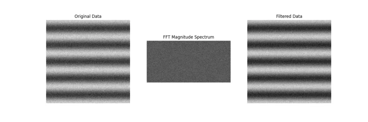
Note: This example is hypothetical and intended for illustrative purposes. The effectiveness of the preprocessing and postprocessing steps would depend on the specific characteristics of your dataset and analysis goals.

Conclusion

The fft.hfft2() function in SciPy is a vital tool for anyone looking to delve into 2D frequency domain analysis, especially with real-world data. Through these examples, we’ve seen its powerful application from simple array transformations to complex image and data analysis tasks. Whether you’re just starting out or are looking to expand your FFT knowledge, fft.hfft2() offers a robust framework for exploring the nuances of Fourier transformations in multi-dimensional data.