Introduction
In the realm of digital signal processing, the Fourier transform is a foundational tool for analyzing the frequencies present in a signal. The fftfreq() function provided by SciPy’s fft module is essential for understanding the frequency components of a discrete Fourier transform (DFT). This article dives into the practical applications of fftfreq() with three illustrative examples, guiding you from basic to more advanced usage.
What does ft.fftfreq() Do?
The fftfreq() function in SciPy generates an array of DFT sample frequencies useful for frequency domain analysis. Whether you’re working with audio data, electromagnetic waves, or any time-series data, understanding how to utilize this function effectively will empower your data analysis and signal processing tasks.
Example 1: Basic Usage of fft.fftfreq()
Let’s start with the most straightforward application of fftfreq(). Here, we aim to obtain the frequency bins for a simple DFT computation.
import numpy as np
from scipy.fft import fft, fftfreq

# Sample parameters
n = 8 # Number of points
T = 1.0 / 800.0 # Sampling period

# Generating sample frequencies
freq = fftfreq(n, T)
print(freq)
Output:
[ 0. 100. 200. 300. -400. -300. -200. -100.]In this instance, the output array freq neatly illustrates the arrangement of sample frequencies for an 8-point DFT, factoring in the sampling period T. This simplistic example lays the groundwork for further exploration and highlights the utility of fftfreq() in frequency analysis.
Example 2: Analysis of Real-world Data
Moving onto a more tangible example, we will analyze a segment of real-world data, demonstrating how fftfreq() can serve to uncover underlying frequency components.
import matplotlib.pyplot as plt
from scipy.fft import fft, fftfreq
import numpy as np

# Loading data (could be from any time-series data source)
data = np.random.randn(1024) # Example data

# Fourier transform and frequency analysis
N = len(data)
T = 1.0 / 800.0
yf = fft(data)
freq = fftfreq(N, T)

# Plotting
plt.plot(freq, np.abs(yf))
plt.title('Frequency Spectrum')
plt.ylabel('Amplitude')
plt.xlabel('Frequency (Hz)')
plt.show()
Output:
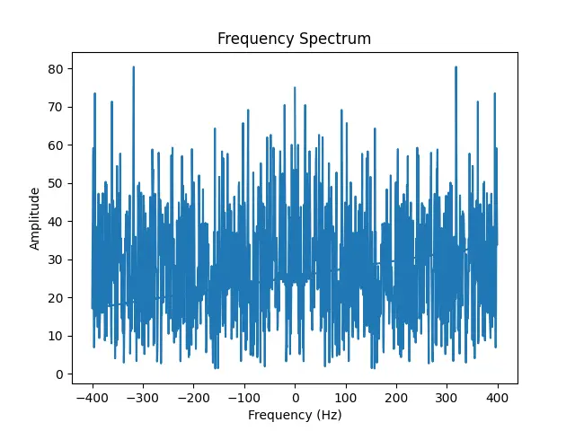
This example provides insight into how frequency analysis via fftfreq() can reveal the amplitude of different frequencies within a given dataset. Such analysis is crucial for tasks ranging from diagnosing machinery based on vibration patterns to analyzing heart rate variability.
Example 3: Complex Signal Analysis
In our final example, we tackle the analysis of a more complex signal, involving multiple frequencies and amplitudes, to demonstrate the capability of fftfreq() in handling sophisticated scenarios.
import matplotlib.pyplot as plt
from scipy.fft import fft, fftfreq
import numpy as np

# Constructing a complex signal
t = np.linspace(0, 1, 1000, endpoint=False)
signal = np.sin(50.0 * 2.0*np.pi*t) + 0.5*np.sin(80.0 * 2.0*np.pi*t)

# Fourier transform of the signal
yf = fft(signal)
freq = fftfreq(1000, 1/1000)

# Visualizing the frequency spectrum
plt.plot(freq, np.abs(yf))
plt.title('Complex Signal Frequency Spectrum')
plt.xlabel('Frequency (Hz)')
plt.ylabel('Amplitude')
plt.show()
Output:
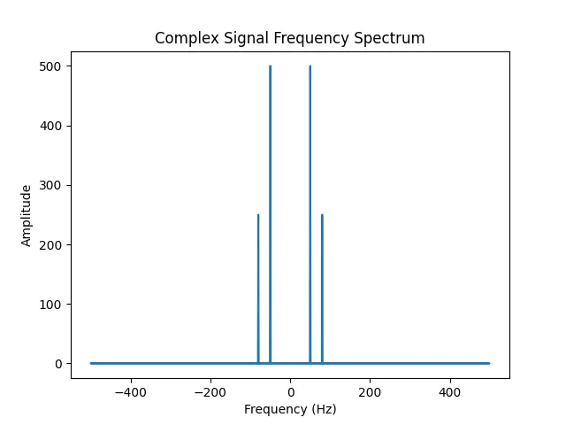
Through analyzing a signal composed of multiple sinusoidal components, this example elucidates how fftfreq() assists in identifying and isolating specific frequencies, a process vital to many engineering and scientific investigations.
Conclusion
The fftfreq() function is a crucial component of the SciPy library, providing an intuitive means for frequency domain analysis in digital signal processing. Through the progression of examples from basic to advanced, we’ve uncovered the function’s versatility and its vital role in uncovering the hidden frequency components in various types of data. Mastering fftfreq() opens doors to a deeper understanding of signals and their characteristics, enhancing both your analysis capabilities and insights.