The Discrete Cosine Transform (DCT) is a key component in signal processing, particularly in data compression, where it’s famed for its use in encoding JPEG images. Python’s SciPy library, with its fft module, offers an accessible interface to perform this transformation through the fft.dct() function. This article will guide you through five progressive examples to master the usage of the fft.dct() function.
Understanding fft.dct()
Before diving into the examples, it’s crucial to understand what fft.dct() does. In essence, the Discrete Cosine Transform transforms a sequence of points (signals or images) into a frequency domain, representing the original data in terms of sum of cosine functions oscillating at different frequencies. SciPy’s fft.dct() function makes this transformation efficient and straightforward.
Example 1: Basic Usage of fft.dct()
To begin with, let’s see how to apply DCT on a simple array.
import numpy as np
from scipy.fft import dct

# Creating a simple array
x = np.array([1, 2, 3, 4])

# Applying DCT
y = dct(x, type=2)  # type=2 is the most commonly used DCT

print('Original array:', x)
print('DCT:', y)
Output:
Original array: [1 2 3 4]
DCT: [20.         -6.30864406  0.         -0.44834153]
The output should is a transformed array, effectively showing the frequency components of the original array.
Example 2: Inverse DCT
Understanding the inverse process is as crucial as the transform itself. The Inverse DCT (IDCT) allows you to retrieve the original data from its frequency representation. Here’s how to perform it:
from scipy.fft import idct

# Assumes y is the result from the previous example
x_reconstructed = idct(y, type=2)

print('Reconstructed array:', x_reconstructed)
Output:
Reconstructed array: [1. 2. 3. 4.]The ability to accurately reconstruct the original array highlights the effectiveness of DCT in lossless transformations and compression applications.
Example 3: DCT on Multi-dimensional Data
Moving beyond one-dimensional arrays, SciPy’s fft.dct() can also handle multi-dimensional data, like images. This example transforms a 2D array, mimicking an image:
import numpy as np
from scipy.fft import dct

# Creating a 2D array (image)
image = np.random.rand(5, 5)  # A random 5x5 image

# Applying DCT on each dimension
image_dct = dct(dct(image.T, type=2).T, type=2)

print('2D DCT:\n', image_dct)
Output:
2D DCT:
 [[ 4.72687475e+01  9.91824519e-01  1.95713338e+00 -2.30595905e+00
   1.05543921e+00]
 [-3.58778240e+00 -2.74318865e+00  6.40046306e-01 -5.21595167e-01
   4.71986439e+00]
   ....
This double application of DCT (once per dimension) effectively processes each dimension separately, a common technique in image processing.
Example 4: Handling Different DCT Types
The fft.dct() function supports different types of DCT, each for specific applications. Here, we’ll use DCT type III, often used for IDCT:
from scipy.fft import dct
import numpy as np

# Creating a simple array
x = np.array([1, 2, 3, 4])
y_type3 = dct(x, type=3)

print('Type III DCT:', y_type3)
Output:
Type III DCT: [11.99962628 -9.10294322 2.61766184 -1.5143449 ]Each DCT type (I, II, III, and IV) has its own usage context, influenced by boundary conditions and the data’s mathematical properties.
Example 5: Advanced Application: Filtering
Finally, an advanced application of fft.dct() in signal or image filtering shows its prowess. Removing high-frequency components can smooth signals or images:
import numpy as np
from scipy.fft import dct, idct

# Example signal
signal = np.random.rand(100)

# Apply DCT
signal_dct = dct(signal)

# Zeroing out high frequencies
threshold = 15
signal_dct[threshold:] = 0

# Apply inverse DCT
smooth_signal = idct(signal_dct)

print('Smoothed Signal:\n', smooth_signal)
Output (vary):
Smoothed Signal:
 [0.53332073 0.52401432 0.50616476 0.48126279 0.45145103 0.41940263
 0.38814899 0.36085668 0.3405613  0.32987676 0.33070734 0.34399772
 0.3695577  0.40599467 0.45077634 0.50043004 0.55086627 0.59779432
 ...
By modifying the DCT coefficients and applying IDCT, we can effectively filter out undesired frequency components, demonstrating DCT’s utility in signal processing.
Conclusion
Through these examples, we’ve explored the fundamental to advanced uses of fft.dct() in Python’s SciPy library. The progression from basic transformations to advanced filtering illustrates the versatility and power of DCT in signal and image processing.
